How to set up a budget in Google Sheets

The trusty spreadsheet is no longer dominated by Microsoft Excel. Google’s offering; Google Sheets, is getting better and better each day. What better way for you to track and improve your finances by setting up a budget using it. In this article, I’ll help you do exactly that, by showing you how to set up a budget in Google Sheets.

How to set up a budget in Google Sheets

Set up an account / login

Firstly, you’ll need a gmail account in order to access the Google Sheets app.

Go to https://www.google.co.uk/sheets/ and you can select the “Personal” -> “Go to Google Sheets” option. At this point, you’ll be asked to sign up or log in to use the service. If you are already signed in, you’ll be taken straight through to the next screen.

Open a new spreadsheet

Now you will be presented with some options to create a new spreadsheet.

If you want a blank spreadsheet for you to customise, select the “Blank” option in the top left.

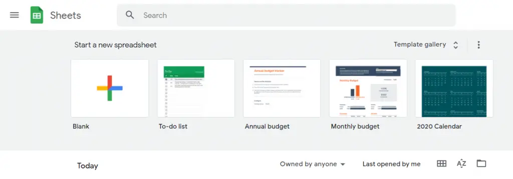
The eagle-eyed amongst you will notice that there are some pre-built templates available within the Google Sheets template already.

One of which is titled “Monthly budget”, and one of which is titled “Annual budget” – ideal. Why reinvent the wheel eh. If you are looking for a pre-made template, these Google default ones are ideal and fairly customisable, with some handy visualisations.

However, if you want a more customisable and simpler spreadsheet of your own, you can simply create your own and build it from there. I’ll cover both here today:

1. Using a pre-designed template
2. Building your own budget in Google Sheets

First, let’s discuss using the pre-designed templates.

Using a pre-designed template

To browse the pre-designed templates available in Google Sheets, press the “Template gallery” to browse them all fully (highlighted below):

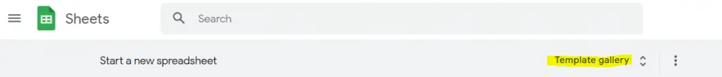
From here you can browse the available templates. Here you should be able to find the two budget templates I was discussing.

• Annual budget
• Monthly budget

Annual budget template

This template looks at your spending and income over a full year.

You can use this template to plan your spend by entering your expected or budgeted values. This will then provide you with a handy view of how much you are expecting to save each month and what that means at a yearly level.

As you go through the year, you can also then overwrite your planned amounts with your actual spend/income.

Enter your expenses and income

To use the template, enter your planned expenses (or actual expenses if the month has already happened) for each category in the tabs “Expenses” and “Income”.

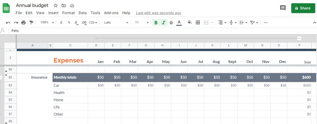
They have quite a comprehensive list of default categories, but if you want to rename or delete certain sub-categories then the summary tab will automatically update. This is because the summary tab automatically calculates the sub-total for that category i.e in the screenshot above it will calculate the total for “Insurance”, and so it doesn’t matter if you rename or delete one of the sub-categories such as “Health” underneath it.

Feel free to update this to fit your finances.

If you wanted to add a completely new category then it will require some changes to the way the spreadsheet has been built, which is out of scope of this article.

Enter your starting balance

On the tab “Setup”, you’ll need to update your “starting balance”. This is your bank balance at the beginning of the year, as it will then apply your expected/planned saving each month (by taking your expected income minus your expected expenses) to provide you a forecast of your expected end of year balance.

Analyse your summary

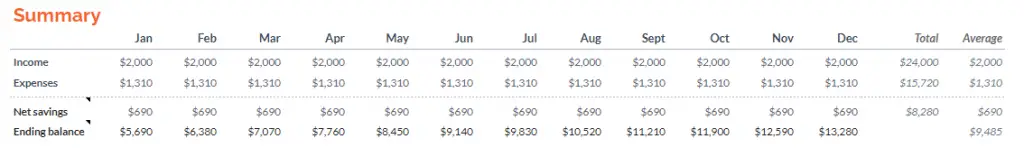
The built-in summary tab provides a handy visualisation of your financial standing over the year, allowing you to easily spot any months where your income is going to be lower than your expenses.

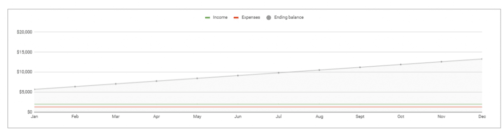
In my example budget above, you can see that I’m expecting my income to be stable each month, and with it my expenses too. So the ending balance of each month is increasing each month by the same amount.

In reality, your budget might be more lumpy, taking account of seasonal up or downswings such as higher spending around Christmas or summer holidays.

The summary tab also summarises your data in a table format. This easily provides you with the view of your income and expenses by month, with your expected savings each month.

The same tab then provides you with similar tables for each sub-category, allowing you to understand where your spending has been increasing.

It would have been nice to see a comparison vs budget/plan over the year, but it would likely become too big a spreadsheet for the time being. I’ll release my own budget template / spend tracker in the near future so subscribe to my blog to stay in the loop when that gets released.

Monthly budget

The second pre-made template that Google have provided is simply called “Monthly budget”.

Rather predictably this template doesn’t look at the full year, but allows you to track your spend and analyse your spend at a monthly level, one month at a time.

Specify your categories and budget

To get started with this template, you need to customise your spend categories and then enter your budgeted/planned spend in each.

Only change the cells that are highlighted. The other cells are all calculated automatically.

Enter your transactions as you go

As you spend, enter your transactions on the “Transactions” tab.

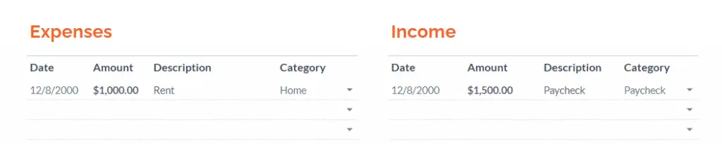
Be sure to enter all of the fields. You can select the category from the dropdown which will reflect your customised categories from the previous step.

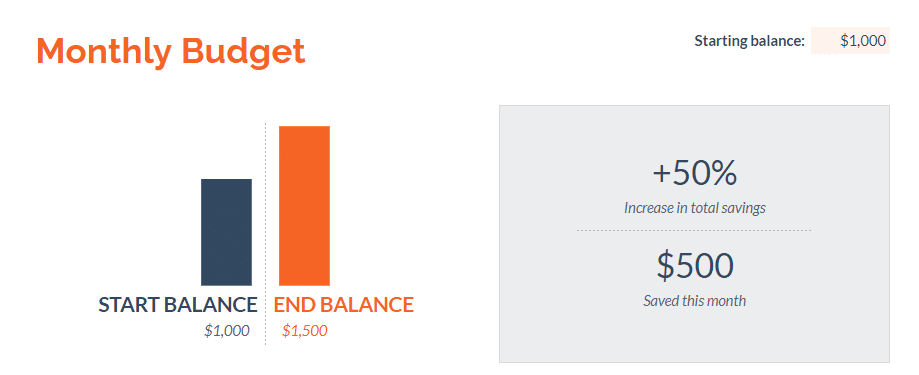
Analyse your spending

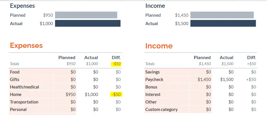
Back on the Summary tab, you’ll see a visualisation looking at your savings.

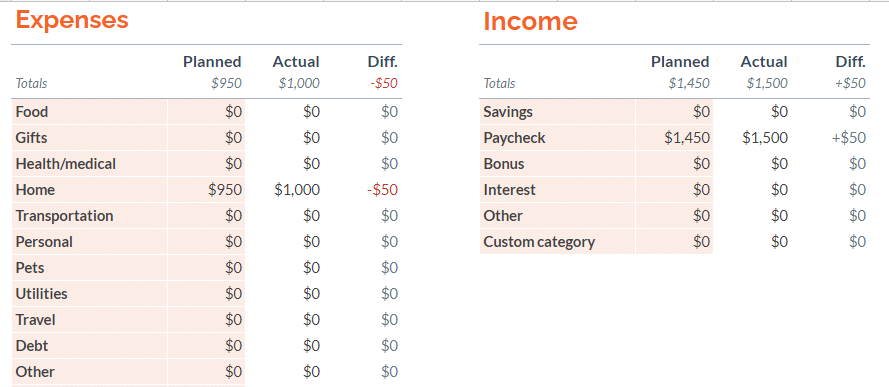
But the great part of this template is the ability to analyse your spending at the category level against your budget.

In the screenshot below, you can see that the actual spend was £50 higher than the budgeted spend. You can then easily identify which line was responsible. In this example, it is the “Home” category that caused it.

Building your own budget

Even though the pre-built templates are handy, they may have too many or too few features for what you need.

Building your own might be the best route for you.

To open a new spreadsheet, navigate back to the Google Sheets dashboard and select “Blank”.

From here, the spreadsheet software is super flexible and will allow you to build up your own budget.

For this example, I’m going to help guide you through the process of building a basic budget which lists your income and expenses, providing you with a calculation of your expected savings and savings rate.

The end result will look like the below. If you want to grab a copy of the file you can make a copy of it for your own use here.

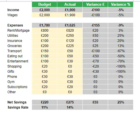
This template can be used to help analyse your actual spend in a month versus your budget. It will help you to easily find the area which has over or under spent and help you to know where to focus for next month.

1. List your income and expense categories

In column B, start listing out your income and expense categories. Be sure to write Income first, then list your different sources of income beneath.

Then do the same by writing Expenses as the sub-category heading and then listing the different expense categories.

You can add as many or as few categories as you want here.

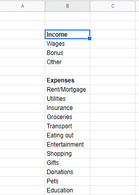
To make the sub-category headings (Income and Expenses) bold, select the cell and then in the ribbon press the “B”.

2. Enter the column headers

Now let’s enter the column headers so we know what data we are looking at.

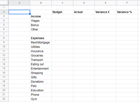
In column C, in the cell in the row above where you put your sub-heading “Income”, put the column header; “Budget”. Then in the same row on column D, enter “Actual”. Then on the same row on column E, enter “Variance £” and on the same row on column F enter “Variance %”.

If you like the style, put these headers in bold too.

It should now look like this:

3. Making the sub-headers automatically calculate their totals

The beauty of using a spreadsheet is through utilising their ability to dynamically update calculations as you go.

We want the spreadsheet to automatically total up our “Income” and “Expense” totals without us needing to do it manually each time we update one of the sub-categories.

To do this, we need to use the =SUM formula. This takes the cells you give it and simply adds them up.

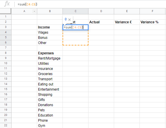
To enter a formula, select the cell as I have done in the below screenshot and type in =SUM(

You will then need to select the cells that you want to be added up. In this example, I’m selecting the cells C4 to C6 (so adding up Wages, Bonus and Other).

Then close the formula with a closing bracket ).

Hit enter and it will calculate.

You will need to do the same for the expense categories too. The only difference will be that you need to select more cells to sum up.

Once you have done that, you can do the same for the “Actual” column.

4. Calculating your net savings

The main reason most people will be trying to track spending and sticking to a budget will be to improve their savings and savings rate. Therefore, these are key metrics to include!

To add this, enter “Savings” and “Savings Rate” underneath your expenses listings.

Then we want to minus your expenses subtotal from your income subtotal.

In the screenshot below, the formula is simply =C3-C8 which is the same as saying:

Savings = Income – Expenses

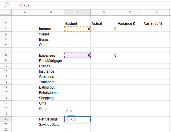
You can do the same for the Actual column (column D i.e cell D20 in the example above).

5. Calculating your savings rate

Expressing your savings as a percentage of your income is a great way to understand how well you are doing given your income level. Generally speaking, a higher percentage is better.

To calculate this, we need to take your net savings and divide it by your income sub-total.

You can see in the example above I’m using the formula =C20/C3 in cell C21. Note that as we are dividing zero by zero, Google Sheets will return an error. Let’s ignore that for now. Once we start entering values for our expenses and income it will start working.

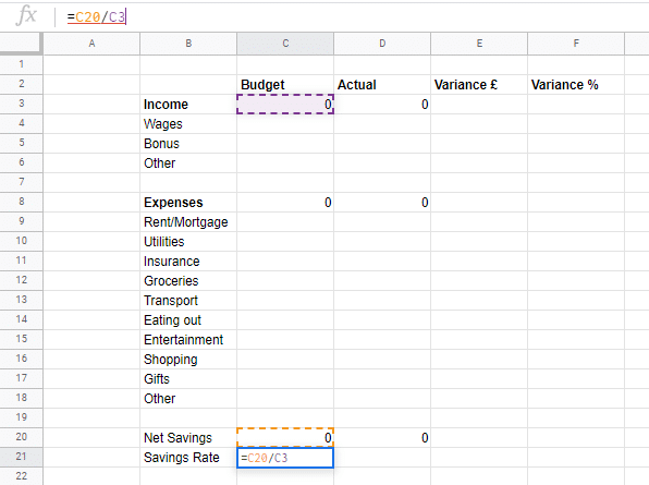
Follow the same for cell D21.

Currently, Google Sheets will display these percentages as a decimal. I.e 10% will be shown as 0.1. If you want it to be displayed as a percentage, then select both cells and select the % sign on the top ribbon. It should look like this:

See related: How to calculate your savings rate

6. Enter your budget

I’m sure you’re itching to get going now. Now that we have the bare bones of the spreadsheet set up, start going through and entering your budget by each category.

Google Sheets will automatically update the sub-totals, net savings and saving rate percentage whilst you fill out your budget.

I’ve entered some dummy numbers, as below:

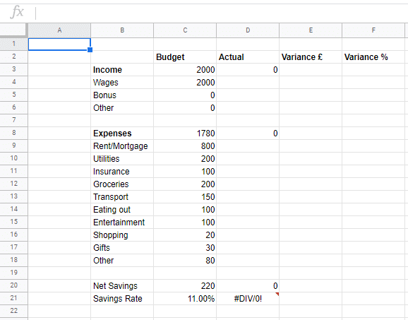
You can see that the savings rate is no longer throwing an error, and is saying that this fictional budget is achieving an 11% savings rate, which is £220 per month.

At this point, the template will allow you to calculate a budget and understand how much money you have left to save each month after all of your expenses are paid for, and what this equates to in a savings rate.

I cover in more detail different budgeting techniques such as the 50/30/20 and line-item budgeting in my article about how to budget your salary wisely.

However, if you want to go one step further and be able to analyse your actual spend versus your budget, then keep on reading.

7. Calculate the difference between your actual spend and your budget

This is really handy to understand where you’ve missed your budget, allowing you to give the problem areas more focus for the following months.

In column E, we want to work out the difference between your actual and your budget, using the formula:

Variance = Actual Spend – Budgeted Spend

In the example below, I can do this in Google Sheets using the formula =D3-C3

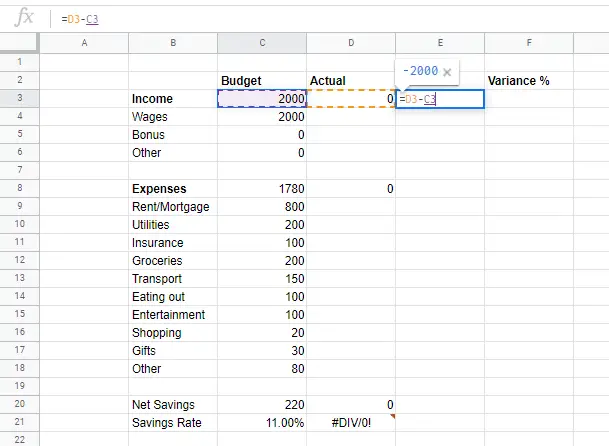
You can do the same for all of the rows with sub-categories as well as just the headings, as this will give you more information to know where you have overspent.

8. Calculate your over or underspend as a percentage

Looking at your over or underspend as a percentage makes it much easier to spot the areas where you missed by a large margin relative to the size of the budget.

To calculate this, we want to divide the variance by the budget.

In this example below, I can do it within Google Sheets by using the formula =E3/C3

Remember to hit the % icon to turn it into a percentage rather than displaying it as a decimal.

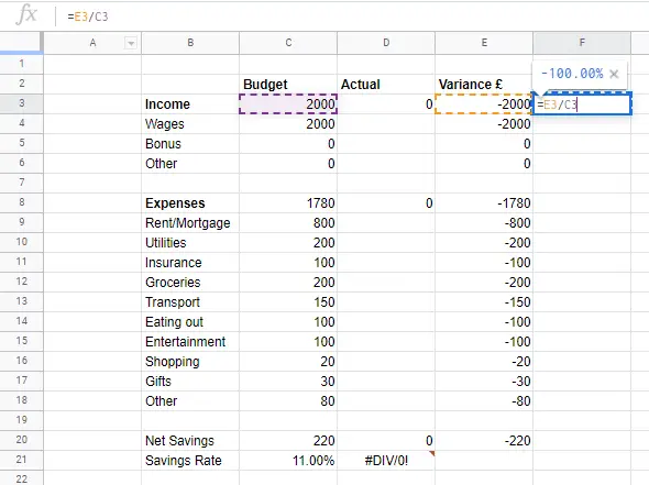
Do the same for all of the sub-categories just like you did with the variance calculation.

9. Enter your actual spend

Once the next month has passed, I’m sure you’ll be itching to see how you did against your budget. Simply enter your actual spend in column D based on the sub-categories. The spreadsheet will automatically calculate your Income and Expense totals, along with your net savings and savings rate metrics.

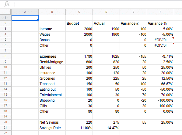
Once you have entered your actual spend, you’ll be able to see how you did against your budget. And helpfully, you’ll see exactly which categories caused an over or under spend.

I’ve entered some dummy figures below, but you can see that total actual savings were £55 higher than was budgeted. Great work to this fiction of my imagination! If you dig into the reason why though, you can see that they actually earned £100 less than they expected.

But they cut back on their expenditure by £155. This was caused mainly by reductions in Transport, Eating Out and Entertainment. Some of their costs actually went up which you would expect to be fairly fixed and easy to forecast such as Rent, Utilities and Insurance which all increased. If this was me, I would start to look at what happened there in the month. If I simply set my budget wrong, I would update my budget to reflect the higher expected spend in future months.

See related: How to save money fast – 13 easy wins you can implement today

10. Bonus: Formatting

Working through to step 9 give you all of the functionality you need for your budget. However, if you want to give it some glitz, then keep reading.

All of the important formatting tools you’ll find in Google Sheets on the ribbon as seen in the screenshot below.

To make a change, you’ll want to select the cell(s) that you want to update and then use the relevant button from the screenshot below in Google Sheets to make the change.

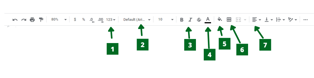
1 – Cell format type. Here you can select whether to present it as a simple number, or as currency (with a currency sign) or as a percentage etc.

2 – Here you can change the font style

3 – In this section, you can make the selected cell Bold and/or Italicised. Even though it doesn’t appear by default, you can also underline content by selecting the right cell and using the shortcut CTRL + U.

4 – This will allow you to change the colour of the text

5 – This will allow you to change the colour of the cell

6 – This will give you the option to add a border to your cell

7 – You can update the alignment of your text. In my version I’ve made all of the headings align to the middle of the cell as I think it looks better

Automated alternatives

Even though you’re wanting to find out how to set up a budget in Google Sheets, I would be doing you a disservice if I didn’t point to some other solutions out there. Rather than having to track your spending manually by entering each transaction into a Google Sheet, you can automate the process using some of the best spend tracking apps on the market.

These can connect to your bank accounts, will automatically categorise transactions and provide insightful visualisations, analytics and sometimes even useful coaching notifications.

The best spend tracking apps I have reviewed previously are:

• Emma review
• Money Dashboard review
• Yolt review

See related: Yolt vs Money Dashboard vs Emma – The Comparison

Conclusion: How to set up a budget in Google Sheets

Google Sheets is a really useful tool to get comfortable with. Like other spreadsheets, Google Sheets gives you the flexibility to manage your finances in a way that fits you best.

Between the two default budget templates and my walkthrough of how to create your own, hopefully, you are well versed now in how to set up a budget in Google Sheets.

If you want to grab a copy of my template that I walked you through above, you can make a copy of it here (to make a copy press File -> Make a Copy).

I hope you enjoyed my article on how to set up a budget in Google Sheets. If you would like to see any other features in the simple budget and spend tracker, let me know in the comments section below.