How to create a personal budget in Excel that’ll even impress your accountant!

When creating a budget, using a spreadsheet app like Excel makes the whole job much, much easier. Today, we’ll look at how to create a budget in Excel, along with a free template I’ve built to help you fill out yours.

As an accountant, I spend most of my time in Excel, and I bloody love it. I’m sure you would have been disappointed if I didn’t advocate the use of Excel at least once! We use Excel for everything from monthly reports tracking business performance, to forecasts and budgets.

If it’s good enough for the world’s largest companies, then it is good enough for us!

I use a spreadsheet to help me set my own budget, as it allows me to tweak my inputs easily to see what the impact will be on my personal profit (the leftover money after all my expenses are paid) without having to manually recalculate.

I also use a spreadsheet as part of my budgeting to analyse my historic spending to see how I’ve been performing versus my budget.

Now I’m sure the idea of analysing your “historic spending” makes you feel sick to your stomach. I promise you it isn’t as bad as it sounds, and using an Excel template like you’re about to learn makes the whole process a LOT easier. Remember, you only need to do a good budget once, the hard bit is then sticking to it!

For those of you who don’t care about building an Excel budget template yourself, I’ve created one for you, which you can download by pressing the link below:

Excel Budget Template - Using Monthly Budget Figures (60 downloads )

However, if you’re wanting to learn how to do it yourself then carry on reading.

I’m going to assume you have little to no experience with Excel, so for the more advanced users feel free to skip ahead to the later steps if I’m going too slow for you.

What will the end result look like?

We want to keep it simple, and show an average monthly budget, along with the two most important metrics;

• Personal Profit (your income minus your expenses).
• Savings rate (this is your personal profit expressed as a percentage of the income you receive).

Want to learn how to build this? Here goes!

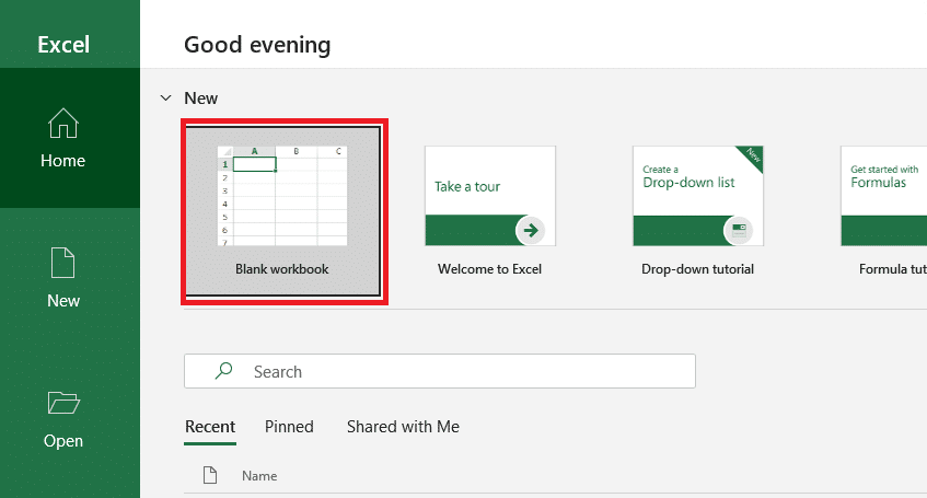
1. Open up your version of Excel and create a new workbook

Once you’ve opened up your version of Excel, you’ll be greeted with a screen like the below. Hit “Blank workbook” to open up a fresh spreadsheet.

If your version just opens straight to a fresh spreadsheet then s’all good, just jump to the next step.

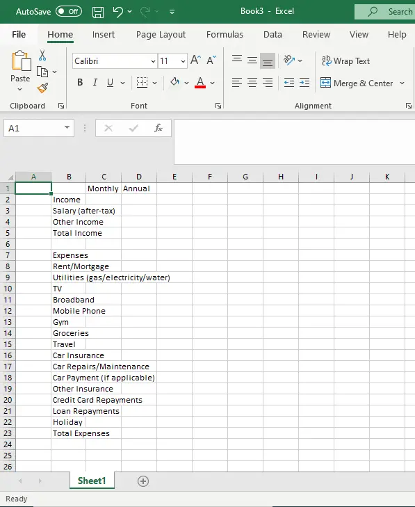
2. Add the main categories in column B

In column B, start listing out the main categories. These will likely vary from person to person so feel free to tweak it, but the default categories I’ve included are as below (including sub-totals).

Income
Salary
Other Income
Total Income

Expenses
Rent/Mortgage
Utilities
TV
Broadband
Mobile Phone
Gym
Groceries
Travel
Car Insurance
Car Repairs/Maintenance
Car Payment
Other Insurance
Credit Card Repayments
Loan Repayments
Holiday
Total Expenses

Of course add in or delete any categories as needed to match your situation.

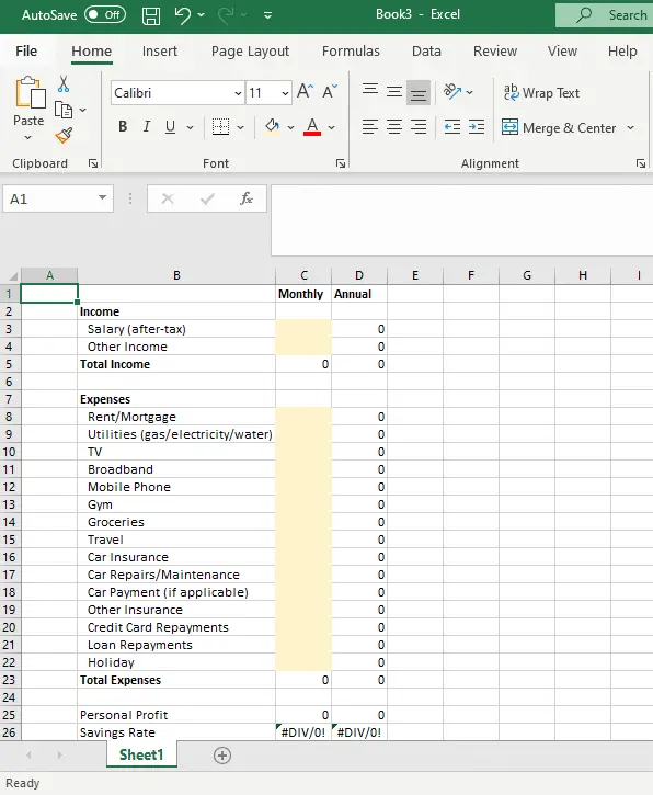
Your workbook should now look like this:

3. Add in the Monthly/Annual columns

We’ll now add in the column titles for the “Monthly” and “Annual” budget. The cells underneath the column for “Monthly” will be the inputs where we will type in our monthly budget, and the annual budget will be calculated automatically.

Add in “Monthly” into cell C1 and “Annual” into cell D1, like so:

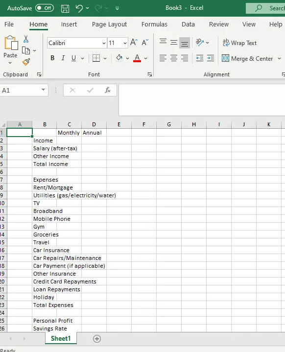
4. Lets add in the metric names

Personal profit (which is the money left over after you deduct all of your expenses from your income), and savings rate (which is your personal profit as a percentage of your income), are the most important metrics for you to track and which you need to optimise your budget for.

To add these, type “Personal Profit” in cell B 25. And in cell B26 type “Savings Rate”, like so:

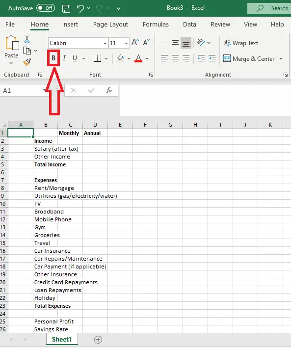
5. Lets format the headings

Now we have the bulk of the content down, we need to format it before we start fleshing out the calculations ready for your budget to be put in.

Select the headings one at a time and press the “B” button on the top ribbon as per below to make the headings bold. The headings to select are cells C1 (“Monthly”), D1 (“Annual”), B2 (“Income”), B5 (“Total Income”), B7 (“Expenses”) and B23 (“Total Expenses”).

It should now look like this:

6. Lets format the category labels (column B)

We want to expand the size of column B so that the text isn’t spilling over the following cells, so when we start filling these in none of the text is obscured.

To do this, hover your mouse over the little line between the column tag “B” and “C” – the mouse should turn to a line with two arrows pointing in opposite directions. Once you have that, double click and it will snap the column to fit the longest content, as below.

Alternatively, hover over the line between B and C as you did before and then manually drag it by holding the mouse down and moving right to increase it until it is as wide as you want it.

7. Add the formulas to automatically calculate the sub-totals

We want Excel to automatically update our totals for “Total Income” and “Total Expenses” whenever we change one of the inputs above them. For example, we want our total expenses sub-total to update if we change our “Groceries” budget. No point in doing that calculation manually if we can save time!

To add the formula for the “Total Income” sub-total, copy and paste the below formula into cell C5:

=SUM(C3:C4)

For the “Total Expenses” sub-total, use the formula:

=SUM(C8:C22)

What this is doing is saying that Excel will take the cells between C8 and C22 and will add them all up, showing the total.

As we have no entries for any of our line items yet, the totals will just show as 0, like below:

8. Add the formula for your Personal Profit metric

We now need to add the formula for our Personal Profit metric, for both the monthly and annual columns.

For the monthly column, copy and paste the following formula into cell C25:

=C5-C23

This formula is simply taking your income sub-total (C5) and deducting the expenses sub-total (C23).

For the annual column, copy and paste the following formula into cell D25:

=D5-D23

9. Add the formula for your Savings Rate metric

For your Savings Rate, copy and paste the following formula into cell C26 for monthly:

=C25/C5

Then press the “%” button which looks like the below:

This will show your savings rate as a percentage rather than a decimal, and is simply showing your personal profit as a percentage of your income.

For your annual column, copy and paste the following formula into cell D26;

=D25/D5

As there are no values, both the monthly and annual formulas will return an error to begin with like below. This is fine and expected at this stage, so don’t worry about it.

Your budget sheet now looks like this:

10. Add the formula for the annual calculations

Once again, Excel can automatically update your annual budget based on your monthly values. No point in us putting it in twice if Excel can do it automatically!

In cell D3, copy and paste the following formula:

=C3*12

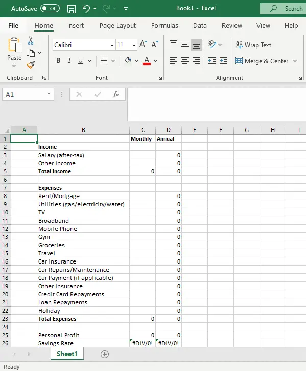
Then within Excel itself, copy the cell D3 by pressing CTRL+C (or right clicking and pressing “Copy”) and then pasting into cells D4, D5 and D8 down to D23.

Your budget sheet will now look like this (the values are 0 as nothing has been entered yet into the “Monthly” column).

11. Highlight the input cells

This is an important habit to get into, as it reminds you when you next come into your template not to change a formula cell.

Highlight cells C3, C4 and C8 down to C22 and select a colour to fill it with using this icon:

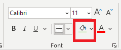
You can select the little downward facing arrow next to it to open up the colour drawer to select the one you want.

I normally use a colour like the below. Your budget sheet should now look something similar to this:

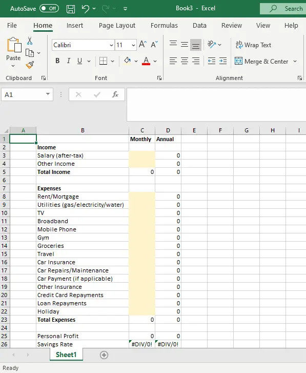
Now that you have the functionality all sorted for your budget sheet, you can start to enter your budget amounts for each item, and see what your personal profit / savings rate is.

I recommend you create this budget using your historic spending information as a guide to see if the budget is realistic, as well as checking our guide for average food budget in the UK to see how you stack up for your groceries line item.

Want to put the finishing touches to your formatting so your excel budget template will become the talk of the town?

12. Indenting the categories

For the categories at the level such as Salary, Rent/Mortgage, TV etc we can indent these so the sub-totals are easier to spot.

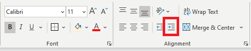
To do this, select these cells and press the indent button as below:

Your budget sheet should now look like this:

13. Using a border

We want to really tidy up our budget by including a border around the main items.

To add a border in excel, you’ll need to first select the cells that you want the border to be around. So for the first section of income categories, select the cells as below:

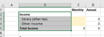
Then select the dropdown on the border icon, and press the “Outside Borders” option. If you prefer, you can select a different style!

Your worksheet will now look like this:

Repeat the process on the groups of cells until your worksheet looks like this. If you ever need to undo something, you can press CTRL+Z.

Note that I’ve also moved cells C1 and D1 down into C2 and D2 to make it neater. You can do this by copying these cells and pasting them in the row below (C2 and D2).

I’ve also included the same “Monthly” and “Annual” column titles in cells C7 and D7 for neatness, but is optional!

14. Removing the grid lines

This is more of a personal preference, but I always prefer it when the grid lines are removed so the worksheet is much neater.

To remove these, navigate to “View” in the ribbon and the section titled “Show”, untick the box for “Gridlines”;

Your worksheet should now look like this:

15. Highlighting the column headers

Purely aesthetic, but highlighting the column headers gives it a nice rounded feel.

I’ve done mine as below, but feel free to tweak the colour scheme to your own tastes! This follows the same instructions as #11.

I hope this tutorial shows you how to create a budget template using excel, letting you loose on this versatile piece of software that will help you create a budget and make tweaks to it quickly and easily.